Designing a Distributed Key-Value Store: The Architectural Blueprint Behind DynamoDB, Cassandra, and Redis
A Beginner-to-Advanced Journey from Single-Node Disk I/O to Resilient Multi-Master Clusters
"Imagine it's 12:00 midnight during a festival flash sale on Amazon or Flipkart. You click 'Add to Cart' on a limited-deal phone. At that exact same second, 200,000 other shoppers across the country click 'Add to Cart' too.
Your screen doesn't freeze with a spinning wheel, and the app doesn't say 'Please wait, database is busy.' In less than 0.005 seconds (faster than a heartbeat), a little green checkmark pops up: 'Item Added to Cart!'
Even if you close the app, switch from your phone to your laptop 2 hours later, or if a severe thunderstorm knocks out power to one of Amazon's datacenter buildings in between — that phone is still sitting safely in your cart.
How does an app record and retrieve millions of these tiny updates instantly without dropping a single item or slowing down?
The secret behind this magic is a Distributed Key-Value Store.
You rarely see it, but it quietly runs behind many of the real-time features you use every day:
* Netflix & Prime Video (The Playback Bookmark Service): When you pause Stranger Things on your living room Samsung TV at 01:24:15, the TV sends a heartbeat write:
playback:usr_98412:stranger_things_s04e09 ➔ {"offset_sec": 5055, "device": "tv", "updated_at": 1728901200}.
When you open Netflix on your iPad in the bedroom 5 minutes later, it fetches that exact key in under 2 milliseconds and prompts: "Resume from 01:24:15". Netflix stores over 100 billion of these bookmarks across global clusters!
* Uber & Swiggy (Real-Time Driver Telemetry): Every 2 seconds, 100,000 active delivery drivers' phones transmit GPS coordinates to a high-speed in-memory store:
driver_loc:blr_koramangala:drv_84102 ➔ {"lat": 12.9352, "lng": 77.6245, "bearing": 184.2, "status": "on_trip"}.
When you open the app to track your food or cab, the system reads this key to animate the little vehicle smoothly across your map in real time.
* Amazon & Flipkart (The Lightning Deal Cart): During a flash sale, you click "Claim Deal". The app shows a 10-minute countdown timer: "Reserved for you! Complete payment in 09:59".
cart:cust_8391024 ➔ {"sku": "APPL-IP16P-256-BLK", "qty": 1, "price": 119900, "ttl_seconds": 600}.
During these 10 minutes, that item is held only for you while other shoppers wait. If you pay in time, the phone is yours. If the timer runs out, the Key-Value store deletes the reservation by itself (this is called TTL / Time-To-Live: "delete this key after 600 seconds"), and the phone goes back to the next shopper. No cleanup job has to scan the main database looking for millions of expired reservations.
* Instagram & WhatsApp (Zero-Friction Authentication): Every time you open Instagram, it doesn't search through a slow database table of 2 billion user accounts. It validates an in-memory session token:
session:auth_tok_89f0a21b ➔ {"user_id": "usr_alex", "auth_status": "active", "expires_at": 1735689600} in less than 1 millisecond.
🗺️ The Scaling Journey: From 1 Computer to a 1,000-Server Fleet
Think of building a Key-Value store like growing a business. You solve challenges one step at a time as traffic explodes:
flowchart LR
    S1["1️⃣ Single Machine<br/><b>Fast Writes</b><br/>Write in 0.001s without disk lag"]
    --> S2["2️⃣ The Fleet<br/><b>Divide the Data</b><br/>Spread keys across 100 servers"]
    --> S3["3️⃣ The Agreement<br/><b>Keep in Sync</b><br/>Prevent data clashes & stale reads"]
    --> S4["4️⃣ Self-Healing<br/><b>Survive Crashes</b><br/>Fix failures automatically"]
    --> S5["5️⃣ Interview Playbook<br/><b>Whiteboard Mastery</b><br/>Ace any 45-min interview"]
Here is the simple story we will follow:
- 1️⃣ The Single Machine: How do we make one computer record data in 0.001 seconds without getting bogged down by slow disks?
- 2️⃣ Spreading the Load: When one computer runs out of space, how do we divide data fairly across 100 computers without a central bottleneck?
- 3️⃣ Keeping Replicas in Sync: When 3 computers hold copies of your cart, how do they agree on what you added if your phone and laptop update at the same instant?
- 4️⃣ Surviving Crashes: Computers reboot and network switches fail all the time. How does the cluster fix itself in the middle of the night with zero human help?
- 5️⃣ The Interview Playbook: How to tie everything together into a clean 5-stage blueprint on a whiteboard during an interview.
Part 1: The Foundations — Single-Node Storage Engine
[!NOTE] What "single-node" means here In Part 1 we zoom in on one machine and ask: how does a single server store and find key-value data quickly and safely? Systems like Cassandra and DynamoDB are distributed (they run on many machines), but every one of those machines runs a storage engine like the one we build here. In Part 2 we connect many of these machines into a cluster.
Step 1: What is a Key-Value Store?
A Key-Value Store is a non-relational database where every record is stored as an exact pairing:
- Key (Unique String): The structured lookup token (e.g.,
"playback:usr_98412:stranger_things","cart:cust_8391024","driver_loc:blr:drv_84102"). - Value (Arbitrary Data): An opaque blob of bytes, plain text, or a serialized JSON object.
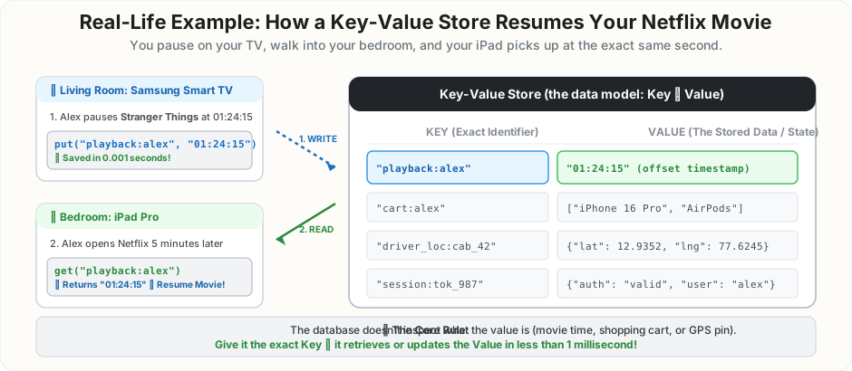
📺 Real-Life Scenario: Resuming Your Netflix Show
Look at the diagram above to see how this works in real life:
1. The Write: Alex pauses Stranger Things on the living room TV at 01:24:15. The TV sends:
put("playback:alex", "01:24:15") ➔ Stored in the Key-Value database in under 0.001 seconds.
2. The Read: Five minutes later, Alex opens Netflix on an iPad in the bedroom. The iPad sends:
get("playback:alex") ➔ The database returns "01:24:15" in 1 millisecond, and the screen prompts: "Resume from 01:24:15".
🏨 Daily Life Analogy: The Hotel Room Keycard Safe
Imagine a 5-star hotel lobby. Behind the reception desk sits a massive wall of numbered electronic safe deposit boxes.
* The Key is the guest’s booking token (e.g., Room-402).
* The Value is whatever the guest places inside that safe (passports, cash, diamond necklace).
* The receptionist doesn't inspect or care what is inside the box. When you present key Room-402, the clerk unlocks that exact box in seconds.
🌉 The Logical Bridge: Why Can't We Just Stop Here?
In Python, you can build a naive Key-Value store in just 2 lines:
Because this lives purely in computer memory (RAM), lookups take less than \(0.0001\) milliseconds (similar to an in-memory cache like Redis).So why can't we just stop here? Why do we need a complex database system?
Because RAM is volatile (temporary)!
If the server restarts, crashes, or trips a power breaker, all customer orders, playback bookmarks, and cart data vanish completely.
| Storage Type | Speed | What Happens When Power Goes Out? |
|---|---|---|
| RAM (Memory) | ⚡ Blindingly fast (\(0.0001\) ms) | 💥 Wiped completely clean! Data vanishes immediately. |
| Disk (SSD / Hard Drive) | 🐢 Slower than RAM | 🛡️ Permanent. Data survives crashes, power cuts, and reboots. |
To build a real-world, fault-tolerant database (like Amazon DynamoDB, Apache Cassandra, or RocksDB), we MUST save our key-value pairs to permanent disk (SSD). But as Step 2 shows, how you write to disk makes a \(100\times\) difference in speed.
Step 2: The Hardware Reality — Why Traditional Databases Freeze on High Writes
Now we face our first big engineering trap:
"Okay, we must write our Key-Value pairs to disk. Why don't we just dump them into a standard relational database like MySQL or PostgreSQL?"
In a system design interview, this is a classic trick question! The answer is NO — we cannot use MySQL or PostgreSQL for massive write workloads.
Understanding why MySQL fails here reveals why dedicated Key-Value stores like Cassandra and DynamoDB were invented in the first place!
1. The Traditional Trap: How MySQL & PostgreSQL Write to Disk (In-Place Overwrites)
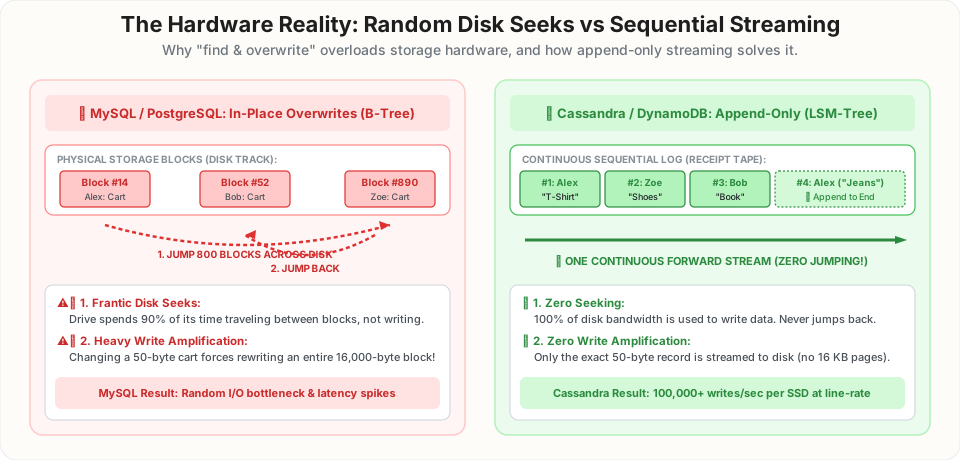
Traditional relational databases (like MySQL or PostgreSQL) organize data into a sorted structure called a B-Tree, divided into fixed chunks called Pages (typically 16 Kilobytes each). Think of it like a printed telephone directory with fixed pages:
When Alex updates his cart: 1. Find: The database searches the disk index to find the exact 16 KB page where Alex's row lives (e.g., Block #14). 2. Read into Memory: It loads the entire 16 KB Page 14 into RAM. 3. Modify: It updates Alex's cart inside RAM. 4. Overwrite in Place: It writes that entire 16 KB page back to that exact physical spot on disk (In-Place Update).
Why Does the Disk Get Overloaded Under High Traffic? (The Two Hardware Killers)
Now imagine 50,000 shoppers checking out at the exact same second during a Black Friday flash sale: * Alex's cart is stored on Block #14 (at the start of the drive). * Zoe's cart is stored on Block #890 (near the end of the drive). * Bob's cart is stored on Block #52 (back near the front).
This triggers two severe hardware penalties:
- 💥 Frantic Disk Seeks: Instead of streaming data smoothly, the disk controller spends 90% of its time jumping back and forth across scattered blocks like a ping-pong ball.
- 💥 Massive Write Amplification: Even if Alex only changed a tiny 50-byte item, the database is forced to rewrite an entire 16,000-byte (16 KB) block back to disk! Writing 16,000 bytes to save 50 bytes wastes huge disk bandwidth.
2. "Wait, Why Doesn't Caching in RAM Prevent the Freeze?" (The Dirty Page Panic)
You might wonder: "Can't MySQL just accept the write in fast RAM (Buffer Pool), tell Alex 'Success!', and save it to disk later in the background?"
Yes! Databases try to do exactly that to stay fast. But during a massive flash sale, this creates a dangerous trap:
- What is a "Dirty Page"?
When Alex updates his cart, the page in RAM has the new cart, but the disk still has the old cart. Any page in RAM with unsaved changes is called a "Dirty Page" (meaning: modified, but not yet permanently saved to disk). - What is "Flushing"?
The database can't keep dirty pages in RAM forever. If power cuts out, all unsaved data is lost. So in the background, the database writes these dirty pages from RAM to disk. This is called Flushing. - The Freeze (When RAM Fills Up):
- On a normal day (50 orders/sec), the database flushes dirty pages calmly in the background.
- But during a flash sale (50,000 orders/sec), new writes arrive faster than the disk can flush them!
- Very quickly, RAM fills up 100% with dirty pages.
- The database runs completely out of memory. It CANNOT accept even one more order!
- The Lock Freeze: The database must pause all incoming checkouts ("Stop! Wait!"). It desperately halts user transactions while trying to flush thousands of scattered pages to disk.
- Because those pages are scattered all over the drive (Block #14, Block #890, Block #52), the disk gets heavily overloaded by random seeks.
- The Crash: A checkout that normally takes 5 milliseconds now takes 10 seconds. Shoppers stare at a spinning wheel, requests time out, and the database crashes!
3. The Key-Value Solution: The Cassandra & DynamoDB Way (Sequential Append)
When engineers at Amazon (building DynamoDB) and Facebook (building Cassandra) saw that traditional B-Trees became overloaded under massive writes, they adopted a radical rule:
Disks are slow at jumping around, but they can stream data at maximum physical line-rate when writing in one straight, continuous line!
The Golden Rule: NEVER search backward. NEVER erase old data. NEVER overwrite in-place!
Instead, treat the disk like a continuous cashier receipt tape (Append-Only Log):
* 10:00 AM → Alex adds "T-Shirt" (appended at the bottom)
* 10:01 AM – 10:59 AM → Thousands of orders from other shoppers stream in...
* 11:00 AM → One hour later, Alex comes back and adds "Jeans" (appended at the current bottom)
Notice the two massive wins: 1. ⚡ Zero Seeking: The storage controller never jumps around. It writes strictly forward in one continuous stream (Sequential I/O). 2. ⚡ Zero Write Amplification: Only the exact 50-byte record is written to disk—no 16 KB block rewrites!
Because 100% of the drive's bandwidth is used for writing data, sequential appending jumps from a few thousand writes to over 100,000 writes per second per SSD (\(100\times\) faster!).
⚖️ Quick Summary: The MySQL Way vs. The Cassandra/DynamoDB Way
| Feature | The MySQL / PostgreSQL Way (SQL) | The Cassandra / DynamoDB Way (Distributed Key-Value) |
|---|---|---|
| Data Structure | B-Tree | LSM-Tree (Log-Structured Merge-Tree) |
| How Data is Written | In-Place Overwrite: Finds the exact 16 KB page and rewrites it. | Sequential Append: Never overwrites; streams only new records to the tail. |
| Disk Behavior | 💥 Random Disk Seeks (Jumps all over the disk). | ⚡ Pure Sequential Streaming (One continuous line). |
| Write Amplification | 💥 High: Changing 50 bytes forces rewriting a 16 KB block. | ⚡ Low: Only the exact 50 bytes are written to disk. |
| Under Heavy Traffic | Memory buffer fills up \(\rightarrow\) System freezes on emergency page flushes. | Writes stay purely sequential \(\rightarrow\) 100,000+ writes/sec per SSD effortlessly. |
🤔 The Million-Dollar Question:
If we never erase old data and only append new lines to the bottom:
1. How do we read Alex's current cart? Alex added a T-Shirt at 10:00 AM. One hour later at 11:00 AM, after 500,000 other people placed orders, Alex added Jeans. When Alex opens his cart to check out, how does the database find his latest cart without scanning through all 500,000 lines from the top?
2. Won't the disk eventually fill up with duplicate, outdated data? His old 10:00 AM cart entry is still sitting on disk taking up space!
Solving these two exact challenges is why the world's fastest databases use the LSM-Tree, which we will explore right now in Step 3!
Step 3: The Secret of Blinding Fast Writes — The LSM-Tree
At the end of Step 2, we were left with two million-dollar questions: 1. If we never erase old data and only append new records to the end of the file, how do we find Alex's latest record without reading through millions of outdated lines? 2. Won't the disk eventually run out of space storing all those old duplicate versions?
The breakthrough solution used by Apache Cassandra, Amazon DynamoDB, Google Bigtable, ScyllaDB, and RocksDB is a specialized storage engine called the LSM-Tree (Log-Structured Merge-Tree).
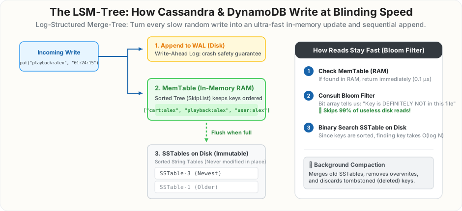
An LSM-Tree solves this by splitting storage into two cooperating layers: fast RAM for instant lookups and sorting, and permanent Disk for sequential append safety.
1. How a Write Works: The End-to-End Walkthrough
Let's follow Alex watching Stranger Things on Netflix. Alex pauses the TV at minute 01:24:15:
When this request arrives at the database, the engine performs two lightning-fast actions in parallel:
Action A: Append to the Write-Ahead Log (WAL) on Disk (Crash Recovery)
- The database immediately writes
playback:alex = 01:24:15to an on-disk, append-only file called the Write-Ahead Log (WAL). - Because this write is strictly sequential (stamped at the tail of the file with zero jumping), it completes in less than 10 microseconds (\(0.01\) ms).
- Why do we do this? If lightning strikes the server 1 millisecond later and power is lost, the server simply replays the WAL upon reboot and recovers Alex's timestamp with zero data loss.
Action B: Insert into the MemTable in RAM (Instant Sorting)
- At the exact same time, the record is placed into an in-memory sorted structure in RAM called the MemTable (implemented as a SkipList or Red-Black Tree).
- Because the MemTable lives entirely in RAM, inserts take less than 0.1 microseconds (\(O(\log M)\) time).
- The MemTable keeps all keys strictly sorted in alphabetical (A–Z) order at all times:
- If a new write arrives right now:
put("balance:alex", "$100"), the MemTable does not tack it onto the end. Because'b'comes before'c', it automatically inserts it at the top to keep everything sorted: - Why keep them sorted? When this memory table is later saved to disk, the resulting file is already sorted A–Z. Searching a sorted file on disk takes only a few quick checks via Binary Search (\(O(\log N)\)) instead of scanning millions of lines!
The Response:
Once written to the WAL and MemTable, the database immediately replies to Alex's TV:
200 OK — Write Successful!(Total latency: under 1 millisecond!)
2. What Happens When RAM Fills Up? (Flushing to SSTables)
RAM is finite (typically sized between 64 MB and 128 MB). When the MemTable fills up:
- The database freezes the current MemTable and opens a fresh, empty MemTable in RAM so incoming user writes never have to wait.
- In the background, a worker thread streams the entire sorted MemTable to disk as an immutable file called an SSTable (Sorted String Table).
- Once the SSTable is safely written to disk, the old WAL can be safely cleared.
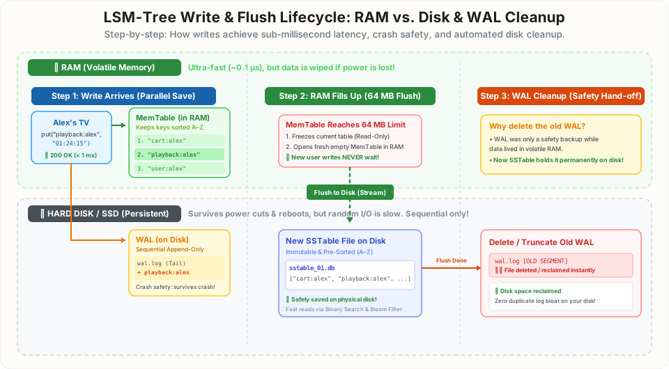
[!IMPORTANT] The Golden Law of SSTables SSTables on disk are 100% IMMUTABLE (never modified, never erased).
If Alex resumes watching and pauses at01:28:00, the engine does NOT modify the existing SSTable on disk. It simply writes the new timestamp into the in-memory MemTable. When that MemTable flushes, a brand-new SSTable file is created on disk containing01:28:00.
3. How Do Deletions Work in an Append-Only Engine? (The Tombstone)
If we can never modify or erase existing files on disk, what happens if Alex clicks "Remove Stranger Things from Continue Watching"?
The database cannot go back into old SSTable files to erase Alex's line. Instead, it writes a special deletion marker called a Tombstone (⚰️):
* playback:alex ➔ ⚰️ TOMBSTONE (Deleted at 10:15 AM)
* This tombstone is appended to the WAL and placed in the MemTable like any normal write.
* When Alex's iPad later asks for get("playback:alex"), the engine sees the tombstone and immediately returns null (Key Not Found / No Saved Bookmark).
* What Netflix Does: Because the bookmark is null, Netflix removes Stranger Things from Alex's "Continue Watching" carousel on his home screen. If Alex chooses to play the show again later, it simply starts from the beginning (00:00:00).
4. How Do Reads Stay Fast? (Bloom Filters & Compaction)
Now consider the read dilemma:
Over time, the database might have 20 different SSTable files on disk. When Alex opens his iPad and requests:
To keep reads lightning-fast, LSM-Trees use two brilliant techniques:
A. The In-Memory Bloom Filter (Skipping Useless Disk Reads)
Every SSTable file on disk has a companion Bloom Filter loaded in RAM: * A Bloom Filter is a tiny, space-efficient bit array (taking only ~10 bits per key). * Before the database opens an SSTable file on disk, it checks the Bloom Filter in RAM: * If the Bloom Filter says "NO", the key is 100% guaranteed NOT to be in that file. The engine skips reading that disk file entirely! * If it says "MAYBE", only then does the engine open that specific SSTable and perform an \(O(\log N)\) binary search. * Result: Bloom Filters eliminate over 99% of unnecessary disk reads!
B. Background Compaction (The Garbage Collector)
What happens to all the old, outdated timestamps (01:24:15) and tombstones sitting in old SSTables?
A quiet background cleaner called Compaction runs continuously:
1. It selects multiple older SSTables (e.g., sstable_01.db and sstable_02.db) and merges them together using the two-pointer merge step (since all input files are already sorted A–Z internally, merging them takes linear \(O(N)\) time instead of an expensive \(O(N \log N)\) sort).
2. For any duplicate keys, it keeps only the newest version (e.g., 01:28:00) and permanently discards the older obsolete versions (01:24:15).
3. It discards tombstoned deleted keys.
4. It writes out one clean, consolidated SSTable and deletes the old, fragmented files from disk.
Part 2: Scaling Out to a Cluster
Step 4: Partitioning Data Across Nodes (Reusing Consistent Hashing)
In Part 1, we designed the storage engine for one single server. But what happens when an application grows to the scale of Amazon or Netflix?
- Storage Limit: A single server can only hold a few Terabytes on its hard drive. An application with hundreds of millions of users might need to store 100 Terabytes. That physically cannot fit on one computer.
- Throughput Limit: A single server's CPU and network card can handle around 50,000 requests per second. During a flash sale, 10 million shoppers click "Add to Cart" at the same second. One machine would be instantly crushed.
To solve this, we must partition (shard) the data across a cluster of dozens or hundreds of machines (e.g., 50 servers holding 2 TB each).
Incoming Request: put("cart:alex", "2 items")
               │
               ▼
       ┌───────────────┐
       │ Hash Function │ ───► Coordinate = hash("cart:alex")
       └───────────────┘
               │
               ▼
       ┌───────────────┐
       │   Hash Ring   │ ───► Walks clockwise to primary node (Node B)
       └───────────────┘
When Alex requests his cart (cart:alex), how does the system know which of the 50 machines holds his data without asking all 50 servers?
As we mastered in Chapter 1:
1. Every physical server is assigned multiple Virtual Nodes (vnodes) around a \(2^{32}-1\) circular hash ring.
2. When a write arrives for cart:alex, the router hashes the key to a coordinate on the ring.
3. The first node encountered walking clockwise is selected as the Coordinator / Primary Replica (e.g., Node B).
4. Adding or removing servers moves only \(\frac{1}{N+1}\) of keys, eliminating catastrophic cache stampedes and massive rebalancing storms.
Step 5: Cluster Topologies — Leader-Follower vs Masterless Leaderless
How should nodes in a cluster coordinate writes and reads? There are two dominant architectural philosophies:
| Feature | Single-Leader / Master-Replica (e.g. Redis, MongoDB) | Masterless / Leaderless (e.g. Amazon Dynamo, Cassandra) |
|---|---|---|
| Write Flow | All writes must go to a designated Master node. Replicas only serve reads. | Any node can accept reads and writes for any key. |
| Single Point of Failure | If the Master node crashes, writes freeze until an election picks a new leader. | Zero single point of failure. Any surviving replica answers writes. |
| Write Throughput | Capped by the CPU/network bandwidth of the single Master node. | Linearly scalable. Add 10 more nodes = get 10x more write throughput. |
| Complexity | Simple mental model (linearized log). | Higher complexity (must handle concurrent write conflicts and quorums). |
For mission-critical applications that can never tolerate write downtime (like Amazon checkout, shopping carts, or messaging queues), the Masterless (Dynamo-style) architecture is the gold standard.
Part 3: Distributed Agreement & Consistency
Step 6: The CAP Theorem & PACELC in Real Systems
Prelude: Why Do Multiple Servers Hold the Same Key? (Replication)
In Step 4, Consistent Hashing placed Alex's data on one server (say, Node 1).
* The Danger: What if Node 1's motherboard catches fire or its hard disk dies? All of Alex's data would be lost forever!
* The Solution (Replication): Every time Alex writes data, the database automatically keeps copies (replicas) on multiple physical servers—for example, Node 1 (New York) and Node 2 (London).
Once two or more servers hold copies of the same data, keeping those copies in sync creates two famous laws of distributed systems: the CAP Theorem and PACELC.
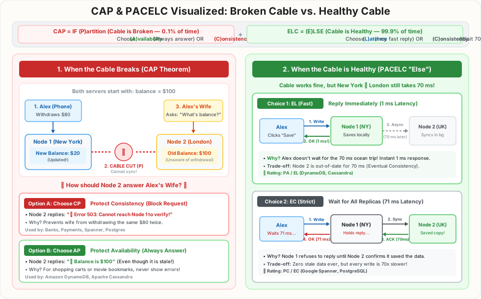
1. What Do the Three Letters of "CAP" Actually Mean?
Before looking at trade-offs, let's define the three letters in plain English:
- C — Consistency (Every Server Shows the Exact Same Data):
If Alex updates his data on Node 1, and 1 second later reads from Node 2, Node 2 must return the newest updated value—never an old, outdated copy. - A — Availability (Every Working Server Always Answers):
Whenever Alex sends a request to any working server, that server must return a valid response. It is never allowed to refuse and throw an "Error 500: Service Unavailable" screen. - P — Partition Tolerance (The Cluster Survives a Broken Network Cable):
A "Network Partition" means the network cable between Node 1 and Node 2 is severed or dropping packets. Both servers are still powered on and users can reach both of them, but Node 1 and Node 2 cannot talk to each other.
2. Why You Can't Have All 3 (The Cut Cable Dilemma)
You have probably heard the common saying: "Pick any 2 out of 3: C, A, or P."
That is misleading! In the real world, network cables will get cut and switches will fail. You cannot "opt out" of network partitions (P is mandatory).
Instead, the real rule of the CAP Theorem is:
When the network cable between servers breaks (\(P\)), you are forced to choose between Consistency (\(C\)) OR Availability (\(A\)).
💳 Concrete Example: Alex's $100 Bank Account vs. Shopping Cart
Suppose both Node 1 (US-East) and Node 2 (US-West) start with balance:alex = $100.
1. ⚡ SNAP! A network failure cuts communication between Node 1 and Node 2 (Partition \(P\)).
2. Alex connects to Node 1 and withdraws \(80**. Node 1 updates his balance to **\)20. (Because the line is dead, Node 1 cannot tell Node 2!)
3. One second later, Alex's wife connects to Node 2 and asks: "What is our account balance?"
Node 2 now faces an unavoidable choice:
| Choice | How Node 2 Responds | What You Gain | What You Sacrifice | Real-World Examples |
|---|---|---|---|---|
| CP (Consistency First) | "My link to Node 1 is down, so I cannot verify if $100 is still accurate. Error 503: Service Unavailable!" | 100% Accuracy (\(C\)): Node 2 never lies or allows withdrawing the same $80 twice. | Availability (\(A\)): Users see error screens and are blocked until the cable is fixed. | Banks, Payments, Stock Inventory (Google Spanner, HBase, ZooKeeper) |
| AP (Availability First) | "My link to Node 1 is down, but I will serve you anyway! Your balance is $100." | 100% Uptime (\(A\)): Users never see an error screen; the app stays up 24/7. | Consistency (\(C\)): Node 2 returns outdated ("stale") data until the cable heals. | Shopping Carts, Netflix Bookmarks (Amazon DynamoDB, Cassandra) |
- Why Banks choose CP: Showing an outdated balance lets someone withdraw money twice. It is safer to show "ATM Out of Service" than lose money.
- Why Amazon Cart & Netflix choose AP: If a network cable breaks, Amazon never wants to block Alex from adding items to his cart, and Netflix never wants to stop Alex from pausing his movie. Serving slightly stale data for a few seconds and syncing later is far better than crashing the app!
3. The PACELC Theorem: What Happens When the Cable is NOT Broken?
Engineers noticed a big gap in the CAP Theorem:
"CAP only tells us what happens during a rare network outage (\(< 0.1\%\) of the year). What about the \(99.9\%\) of the time when all network cables are working perfectly?"
Even when the cable between Node 1 (New York) and Node 2 (London) is healthy, it still takes ~70 milliseconds for data to travel across the ocean.
When Alex clicks "Save" on Node 1 during normal operation, Node 1 still has to make a trade-off between Latency (\(L\) = Fast Speed) and Consistency (\(C\)):
- Option 1: Choose Low Latency (\(L\)) — Reply Immediately:
Node 1 saves Alex's data locally, immediately replies200 OKto Alex in 1 millisecond, and copies the data to Node 2 in the background. - Result: Blindingly fast user experience (Low Latency), but for 70 ms Node 2 is slightly behind (Eventual Consistency).
- Option 2: Choose Strong Consistency (\(C\)) — Wait for All Replicas:
Node 1 sends the update across the ocean to Node 2 and forces Alex to wait 70 milliseconds until Node 2 confirms it saved the copy before replying200 OK. - Result: Node 1 and Node 2 are 100% in sync at every millisecond (Strong Consistency), but every write is much slower (High Latency).
Combining both situations gives the 6 letters of the PACELC Theorem:
IF there is a (P)artition (Network cable is broken):
    Choose between (A)vailability   OR   (C)onsistency
(E)LSE (Network is healthy 99.9% of the time):
    Choose between (L)atency (Speed) OR  (C)onsistency
⚖️ PACELC Cheat Sheet for Real Databases
| Database | PACELC Rating | If Cable Breaks (P) | When Network is Healthy (E) | Best Used For |
|---|---|---|---|---|
| Apache Cassandra | PA / EL | A: Stay online (never error) | L: Reply in 1 ms (sync in background) | High-speed chat, telemetry, feeds |
| Amazon DynamoDB | PA / EL | A: Stay online (never error) | L: Reply in single-digit ms | Shopping carts, user sessions, profiles |
| Google Cloud Spanner | PC / EC | C: Block stale reads/writes | C: Wait for replicas to confirm | Banking ledgers, billing, inventory |
| MongoDB / Postgres | PC / EC | C: Block isolated nodes | C: Read/write strictly via Primary | Transactional business data |
Step 7: Quorum Consensus Mathematics (\(W + R > N\))
In a masterless system, how do we guarantee that a client reading data gets the most up-to-date value, even if some nodes haven't finished replicating yet?
We use Quorum Consensus.
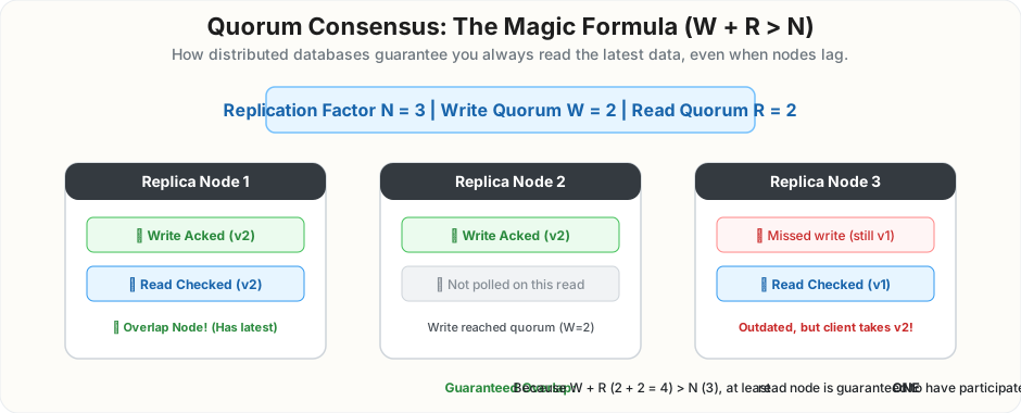
We configure three variables: * \(N\): The Replication Factor (total number of distinct servers that store a copy of the key, typically \(N = 3\)). * \(W\): The Write Quorum (how many nodes must acknowledge a write before we declare success to the client). * \(R\): The Read Quorum (how many nodes the coordinator must poll when reading data).
The Golden Overlap Rule:
If the sum of nodes written to (\(W\)) and nodes read from (\(R\)) is strictly greater than the total number of replicas (\(N\)), the Pigeonhole Principle guarantees that at least ONE node in your read set participated in the most recent write set!
🔢 Concrete Numerical Example:
Suppose \(N = 3\), \(W = 2\), and \(R = 2\):
1. A client writes "status": "shipped".
2. The coordinator sends writes to Node 1, Node 2, and Node 3.
3. Node 1 and Node 2 acknowledge immediately. Node 3 is experiencing a temporary network hiccup and lags behind.
4. Because \(W = 2\), the coordinator sends 200 OK to the client.
5. Later, another user reads "status". The coordinator polls any 2 nodes (e.g., Node 1 and Node 3).
* Node 1 returns "status": "shipped" (timestamp \(T_2\)).
* Node 3 returns "status": "pending" (timestamp \(T_1\)).
6. Because Node 1 has a newer timestamp (\(T_2 > T_1\)), the coordinator returns "shipped" to the user, and asynchronously sends a background update to repair Node 3 (Read Repair)!
Tunable Consistency Knobs:
| Configuration | Tradeoff | Best For |
|---|---|---|
| \(W = 1, R = N\) | Blazing fast writes, slower reads | High write-volume telemetry & IoT sensors |
| \(W = N, R = 1\) | Slower writes, ultra-fast single-node reads | High-read caches with infrequent writes |
| \(W = 2, R = 2\) (\(N=3\)) | Balanced low latency with strong consistency (\(W+R > N\)) | Production default for general databases |
Step 8: Concurrent Conflicts — Last-Write-Wins (LWW) vs Vector Clocks
In a masterless distributed system, any server can accept writes. But what happens if two updates to the same key happen at the exact same millisecond across different nodes?
📱 The Real-Life Scenario: Alex on Two Devices at Once
Imagine Alex is shopping on Amazon. His cart initially contains a pair of ["Shoes"] (stored on Node A).
At 10:00:00 AM, Alex is browsing on both his phone and his laptop:
1. On his Phone (connected to Node B): Alex clicks "Add Shirt".
\(\rightarrow\) Node B saves: cart:alex = ["Shoes", "Shirt"].
2. On his Laptop (connected to Node C): At the exact same second, Alex clicks "Add Hat".
\(\rightarrow\) Node C saves: cart:alex = ["Shoes", "Hat"].
Because Node B and Node C are in different data centers and haven't communicated yet, neither node knows what the other just did!
Now, at 10:00:05 AM, Alex opens his iPad to check out. The iPad asks the database for cart:alex.
* Node B returns: ["Shoes", "Shirt"]
* Node C returns: ["Shoes", "Hat"]
The database faces a massive conflict: Which cart is the real truth? * If it arbitrarily chooses Node B \(\rightarrow\) The Hat mysteriously disappears from Alex's cart! * If it arbitrarily chooses Node C \(\rightarrow\) The Shirt mysteriously disappears from Alex's cart!
In an e-commerce platform, silently deleting items from a customer's cart causes customer anger, abandoned checkouts, and millions of dollars in lost revenue.
How does a distributed database resolve this? There are two primary philosophies:
Approach 1: Last-Write-Wins (LWW) — The Blind Guess (Used by Cassandra)
Under Last-Write-Wins (LWW):
* Every time a write happens, the server attaches a physical wall-clock timestamp (from NTP).
* When a conflict occurs between Node B and Node C, the coordinator looks at both timestamps:
* Node B timestamp: 10:00:00.100 AM
* Node C timestamp: 10:00:00.105 AM
* Node C is 5 milliseconds "later", so Node C wins! The cart becomes ["Shoes", "Hat"], and Node B's write is permanently thrown in the trash.
Approach 2: Vector Clocks — The Smart Merge (Used by Amazon Dynamo)
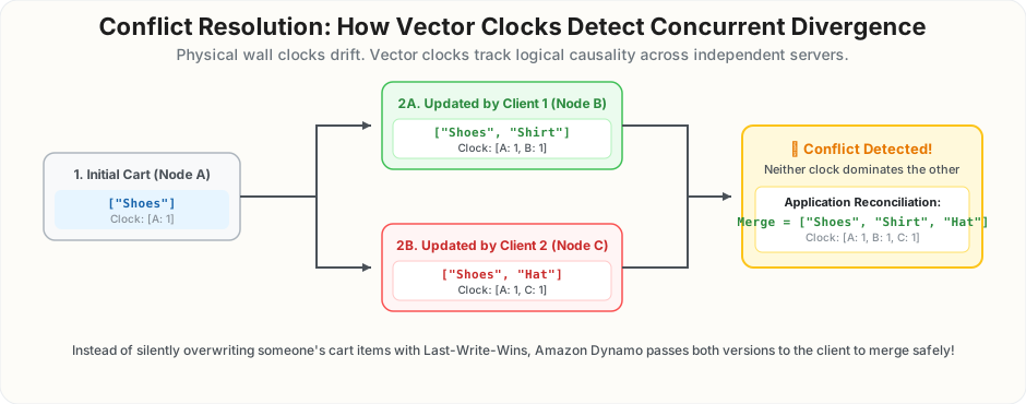
Instead of trusting unreliable physical wall clocks, Amazon Dynamo invented Vector Clocks to track the logical cause-and-effect relationship (causality) between writes.
A Vector Clock is a list of (NodeID, Counter) version stamps attached to every record, like a passport that gets stamped by every server it visits:
The Step-by-Step Walkthrough:
-
Step 1: The Initial Cart (Node A)
Alex's cart contains["Shoes"]. Node A stamps its counter: $\(\text{Cart: } \mathbf{["Shoes"]} \quad | \quad \text{Clock: } \mathbf{[A: 1]}\)$ -
Step 2A: Phone Write (Node B)
Alex adds "Shirt" via his phone. Node B receives the cart with clock[A: 1], adds "Shirt", and appends its own stamp: $\(\text{Cart: } \mathbf{["Shoes", "Shirt"]} \quad | \quad \text{Clock: } \mathbf{[A: 1, B: 1]}\)$ -
Step 2B: Concurrent Laptop Write (Node C)
Simultaneously, Alex adds "Hat" via his laptop. Node C also received the original cart with clock[A: 1], adds "Hat", and appends its own stamp: $\(\text{Cart: } \mathbf{["Shoes", "Hat"]} \quad | \quad \text{Clock: } \mathbf{[A: 1, C: 1]}\)$ -
Step 3: Conflict Detection on the iPad
When Alex's iPad requestscart:alex, the coordinator receives both versions: - Version 1:
[A: 1, B: 1] - Version 2:
[A: 1, C: 1]
The database compares the vector clocks:
* Is Version 1 strictly newer than Version 2? No (it has B: 1, but lacks C: 1).
* Is Version 2 strictly newer than Version 1? No (it has C: 1, but lacks B: 1).
* Conclusion: Neither write knows about the other. A concurrent branch (fork) has occurred!
- Step 4: Application Reconciliation (The Merging Magic)
Instead of guessing or deleting data, the database refuses to throw either version away! It preserves both versions (called siblings) and passes them up to the Amazon shopping application:"Hey Amazon App: Alex has two conflicting versions of his cart. Please reconcile them!"
The shopping application knows the business logic: items added to a cart should never be lost. It takes the union of both carts: $\(\text{Merged Cart} = \mathbf{["Shoes", "Shirt", "Hat"]}\)$
- Step 5: Write Back the Merged State
The application writes the merged cart back to the database with a merged vector clock: $\(\text{Cart: } \mathbf{["Shoes", "Shirt", "Hat"]} \quad | \quad \text{Clock: } \mathbf{[A: 1, B: 1, C: 1]}\)$
Alex sees all three items in his cart, checks out happily, and zero data was lost!
⚖️ Comparison: Last-Write-Wins vs Vector Clocks
| Feature | Last-Write-Wins (LWW) | Vector Clocks |
|---|---|---|
| Used By | Apache Cassandra, ScyllaDB | Amazon DynamoDB, Riak |
| How Conflicts are Handled | Compares physical timestamps; highest wall clock silently discards the other. | Detects concurrent branches; preserves both versions (siblings). |
| Risk of Data Loss | 💥 High (clock skew causes silent overwrites). | 🛡️ Zero (no data is ever deleted automatically). |
| Complexity | Simple and fast (no merging logic required). | Requires application-level reconciliation logic to merge siblings. |
| Best Used For | Idempotent sensor metrics, GPS telemetry where latest value always replaces old. | Mission-critical user data (Shopping carts, financial balances, profile settings). |
Part 4: Self-Healing & Failure Recovery
Step 9: Decentralized Failure Detection — The Gossip Protocol (SWIM)
In a 500-node cluster, how does every node know which machines are alive and which have crashed, without a centralized master or controller?
Distributed databases use a decentralized Gossip Protocol (based on the academic SWIM algorithm):
         ┌────────┐
         │ Node A │
         └───┬────┘
             │
     Random  │ "Node C heartbeat is 42"
     Gossip  ▼
         ┌────────┐
         │ Node B │ ────► Gossips to Node D and Node E...
         └────────┘
- Every second, each node randomly picks a small number of random peers (typically 3 nodes) and exchanges a list of known cluster states and incrementing heartbeat counters.
- If Node C's heartbeat counter stops increasing for a predetermined suspicion window:
- Node A marks Node C as "Suspect".
- Node A gossips to peers: "Has anyone heard from Node C?"
- If no peer hears from Node C within a grace period, Node C is declared "Dead".
- Result: Failure information spreads through a 1,000-node cluster exponentially in \(O(\log N)\) time, consuming negligible network bandwidth without any central master bottleneck!
Step 10: Temporary Server Outages — Sloppy Quorums & Hinted Handoff
What happens if Node A (one of the 3 designated replicas for a key) is briefly rebooting for an OS patch, and a client tries to write to it?
If the database strictly required Node A, the write might fail or violate quorum.
Instead, Amazon Dynamo invented Sloppy Quorum with Hinted Handoff:
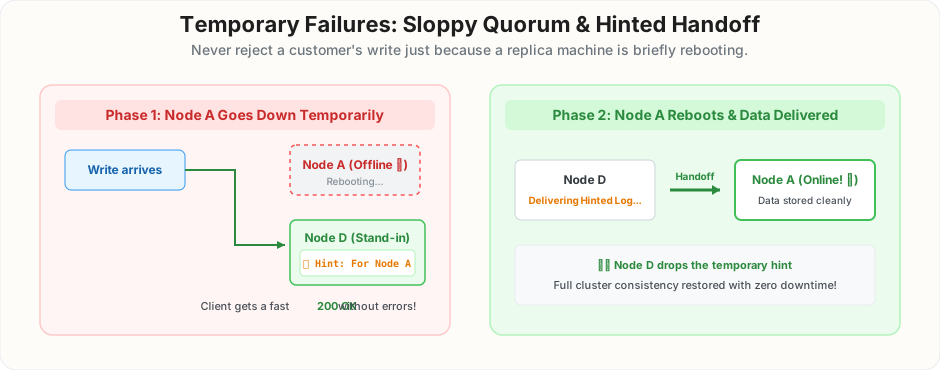
- The coordinator detects that primary replica Node A is unreachable.
- Instead of failing the write, the coordinator finds the next healthy server on the hash ring (say, Node D).
- Node D accepts the write, but attaches a metadata tag:
[HINT: This data belongs to Node A. Store temporarily.] - The write succeeds and the client receives a fast
200 OK. - In the background, Node D monitors Node A via the Gossip protocol.
- As soon as Node A comes back online, Node D streams all stored writes back to Node A (Handoff), and deletes its temporary local copy.
- Result: High availability for writes even during partial network outages!
Part 5: Interview Mastery & Summary Blueprint
Step 11: The 5-Stage System Design Interview Blueprint
If an interviewer asks:
"Design a Distributed Key-Value Store like Amazon DynamoDB or a Distributed Cache"
Follow this battle-tested 5-stage blueprint on the whiteboard:
┌─────────────────────────────────────────────────────────────────────────────┐
│             SYSTEM DESIGN INTERVIEW BLUEPRINT: KEY-VALUE STORE              │
├─────────────────────────────────────────────────────────────────────────────┤
│ 1. Clarify Requirements & Scope:                                            │
│    • Operations: get(k), put(k, v), delete(k)                               │
│    • Scale: 10M+ QPS, sub-10ms latency, high availability                   │
│    • Consistency: Tunable (Eventual vs Strong Consistency)                  │
│                                                                             │
│ 2. Storage Engine (Single Node):                                            │
│    "To avoid slow random disk I/O, I'll use an LSM-Tree architecture:       │
│    Write-Ahead Log (WAL) on disk for durability + MemTable in RAM for speed.│
│    Flush sorted immutable SSTables to disk, with Bloom Filters to eliminate │
│    99% of unnecessary disk seeks on reads."                                 │
│                                                                             │
│ 3. Partitioning & Data Placement:                                           │
│    "Use Consistent Hashing with 100-256 virtual nodes per server to         │
│    distribute keys uniformly across the cluster and prevent hot arcs.       │
│    Replicate each key to N distinct physical servers clockwise."            │
│                                                                             │
│ 4. Consistency & Replication Strategy:                                      │
│    "Adopt a masterless leaderless architecture. Enforce Quorum Consensus    │
│    (W + R > N) so reads always overlap with writes. Use Vector Clocks to    │
│    detect concurrent branching conflicts instead of losing data to LWW."    │
│                                                                             │
│ 5. Failure Handling & Self-Healing:                                         │
│    "Decentralized failure detection via Gossip Protocol (SWIM). Handle      │
│    temporary server outages with Sloppy Quorums and Hinted Handoff so       │
│    writes never fail when a replica reboots."                               │
└─────────────────────────────────────────────────────────────────────────────┘
Step 12: Summary Cheat Sheet
| Distributed Component | Primary Technique | Production System | Core Benefit |
|---|---|---|---|
| Write Performance | LSM-Tree (WAL + MemTable + SSTable) | Cassandra, RocksDB, Bigtable | Turns slow random disk I/O into fast RAM inserts + sequential disk appends |
| Fast Reads | Bloom Filter (Probabilistic bit array) | RocksDB, Cassandra | Skips 99% of unnecessary disk reads for keys not in an SSTable |
| Partitioning | Consistent Hashing + Vnodes | DynamoDB, Cassandra | Distributes keys evenly across servers with minimal movement on resize |
| Read/Write Consensus | Quorum (\(W + R > N\)) | Dynamo, Cassandra | Guarantees read and write replica sets overlap by at least 1 server |
| Conflict Resolution | Vector Clocks / Sibling Merging | Dynamo, Riak | Detects concurrent writes and merges versions without losing user data |
| Failure Detection | Gossip Protocol (SWIM) | Cassandra, Consul | Decentralized peer-to-peer health checks with no single point of failure |
| Temporary Outages | Sloppy Quorum & Hinted Handoff | DynamoDB, Cassandra | Neighbor server holds missed writes temporarily until rebooting node returns |