Sampling Parameters Explained: How Temperature, Top-K, and Top-P Control What an LLM Says Next
A Step-by-Step Guide to How an AI Picks Its Next Word, Why Random Guesses Happen, and How to Control Its Creativity
The Question Left Over from Chapter 2: How Does the AI Pick One Winning Word?
In Chapter 2 (Tokens & Embeddings), we traced what happens when Alex types:
"Please check the latest Apple ___"
We saw how the computer chops those words into Tokens, maps their meaning into Embeddings, and runs them through its attention layers.
At the very end of that process, the AI does not output a single finished word. Instead, it scores every word in its 200,000-word dictionary and hands back a list of possibilities for what could fill in the blank:
- "stock" ➔ 45% chance
- "price" ➔ 30% chance
- "earnings" ➔ 15% chance
- "revenue" ➔ 7% chance
- "pie" ➔ 3% chance
That leaves us with a puzzle: How does the computer actually pick ONE word from that list?
At first glance, there are two obvious ways to do it—and both have major flaws:
-
Choice A: Always pick the #1 highest percentage ("stock", 45%) This sounds safe, but it makes the AI completely rigid. If Alex asks for three creative tagline ideas or a brainstorming list, the AI will produce the exact same robotic output every time. Worse, models picking only the top word often get trapped in loops, repeating the same phrase over and over ("the price of the stock of the price of the stock...").
-
Choice B: Roll dice using the percentages ("stock" 45%, "price" 30%, "pie" 3%) Now the AI has variety! Most of the time it picks a sensible word like
"stock"or"price". But in a dictionary of 200,000 words, hundreds of strange or irrelevant words still have a 1% or 2% chance. On an unlucky roll, the dice land on that 3% chance for"pie"—and Alex's financial bot confidently announces: "Sure! Checking the latest Apple pie coming right up!"
This is the central dilemma of text generation:
Always picking the top word is too robotic. Rolling dice across every word is too reckless.
To get the sweet spot—natural variety without nonsense words—every LLM provides three control dials called Sampling Parameters: Temperature, Top-K, and Top-P.
[!NOTE] Short Answer (30-Second Summary) Once the AI calculates probabilities for the next word, Sampling Parameters decide how the winner is chosen:
- Temperature (The Adventure Dial): Controls how wild or cautious the AI is.
- Low (0.0 – 0.2): Always picks the safest, most obvious word. Best for math, code, and exact facts.
- High (0.8 – 1.0+): Gives less obvious words a fighting chance. Best for brainstorming and creative writing.
- Top-K (The Fixed Headcount): Keeps a fixed number of words (for example,
Top-K = 3keeps only"stock","price", and"earnings"), completely ignoring the rest of the dictionary.- Top-P (The Quality Threshold): Keeps words until their combined chances add up to \(P\) percent (for example,
Top-P = 0.90). For Alex's prompt "Please check the latest Apple ___", it gathers"stock"(45%) +"price"(30%) +"earnings"(15%) = 90%, keeping the 3 sensible financial words while automatically throwing away the 3% chance of"pie".
How Token Sampling Works Internally
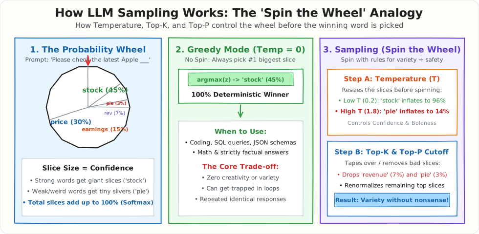
Imagine a spinning prize wheel where each slice is a candidate word:
- Slice size = Confidence: Strong words get giant slices (
"stock"gets a huge 45% slice), while weird words get tiny slivers ("pie"gets just 3%). - Greedy Mode (No Spin): You don't spin the wheel at all. You just grab the biggest slice every single time (
Temperature = 0). It is 100% predictable, but can get boring and robotic. - Sampling Mode (Spin the Wheel): You spin the wheel to allow variety, but use rules to keep it safe:
- Temperature resizes the slices (low temperature makes the biggest slice even bigger; high temperature makes all slices more equal).
- Top-K and Top-P remove the bad slices entirely before the spin, so the pointer can never land on
"pie".
Let's trace the exact math step by step.
1. From Raw Logits to Softmax Probabilities
When the final Transformer layer finishes processing Alex's prompt ("Please check the latest Apple ___"), it outputs an array of 200,000 raw, unnormalized floating-point numbers called Logits (\(z\)).
Logits are not percentages yet. They can be positive (+3.2), exactly zero (0.0), or strongly negative (-2.5, -6.0). To turn raw logits into clean percentages that add up to 1.0 (100%), the engine passes them through the Softmax function:
Why use exponents (\(e^{z_i}\)) instead of just dividing by the sum?
1. Logits can be negative or zero, but probabilities cannot: Exponentiating any real number—positive, zero, or negative—always produces a strictly positive value (\(e^z > 0\)).
2. Exponentiating amplifies strong scores: A logit of 3.2 becomes \(e^{3.2} \approx 24.53\), while a logit of 0.5 becomes \(e^{0.5} \approx 1.65\).
Step-by-Step Math: How Does 'stock' Turn into 45%? (Click to expand)
Suppose the AI finishes evaluating Alex's prompt ("Please check the latest Apple ___") and outputs these raw logits (\(z\)):
"stock": \(z = 3.2\)"price": \(z = 2.8\)"earnings": \(z = 2.1\)"revenue": \(z = 1.3\)"pie": \(z = 0.5\)
The engine runs the Softmax calculation in 3 steps:
1. Step 1: Calculate the exponent (\(e^z\)) for every candidate:
- \(e^{3.2} \approx \mathbf{24.53}\)
- \(e^{2.8} \approx \mathbf{16.44}\)
- \(e^{2.1} \approx \mathbf{8.17}\)
- \(e^{1.3} \approx \mathbf{3.67}\)
- \(e^{0.5} \approx \mathbf{1.65}\)
2. Step 2: Sum all exponents together (The Denominator):
3. Step 3: Divide each word's score by the total sum:
"stock": \(\frac{24.53}{54.46} = 0.4504 \longrightarrow \mathbf{45\%}\)"price": \(\frac{16.44}{54.46} = 0.3018 \longrightarrow \mathbf{30\%}\)"earnings": \(\frac{8.17}{54.46} = 0.1500 \longrightarrow \mathbf{15\%}\)"revenue": \(\frac{3.67}{54.46} = 0.0674 \longrightarrow \mathbf{7\%}\)"pie": \(\frac{1.65}{54.46} = 0.0303 \longrightarrow \mathbf{3\%}\)
Notice that while the raw score difference between "stock" (\(3.2\)) and "pie" (\(0.5\)) is only \(2.7\), exponentiation amplifies that gap (\(24.53\) vs. \(1.65\)), making "stock" 15 times more likely to win than "pie".
What Do Positive, Zero, and Negative Logits Mean?
| Logit Type | Example Word | Raw Logit (\(z\)) | Exponent (\(e^z\)) | What It Means in Plain English |
|---|---|---|---|---|
| Strong Positive | "stock" |
+3.2 |
\(e^{3.2} \approx 24.53\) | Strong semantic match with context. |
| Mild Positive | "earnings" |
+1.5 |
\(e^{1.5} \approx 4.48\) | Plausible word, moderate match. |
| Neutral Zero | "pie" |
0.0 |
\(e^{0.0} = \mathbf{1.0}\) | Baseline. A logit of 0.0 does not mean 0% chance! It gets an unnormalized score of 1.0. |
| Negative Logit | "banana" |
-2.5 |
\(e^{-2.5} \approx \mathbf{0.082}\) | Semantic mismatch. Exponent is tiny, but still strictly positive. |
| Strongly Negative | "spaceship" |
-6.0 |
\(e^{-6.0} \approx \mathbf{0.0025}\) | Completely irrelevant token. Probability is near-zero. |
2. How Temperature (\(T\)) Reshapes the Curve
Before running Softmax, the engine divides every raw logit \(z_i\) by a number called Temperature (\(T\)):
Let's see what dividing by \(T\) does to 5 candidate tokens for "Please check the latest Apple ___" with raw logits stock = 3.2, price = 2.8, earnings = 2.1, revenue = 1.3, and pie = 0.5:
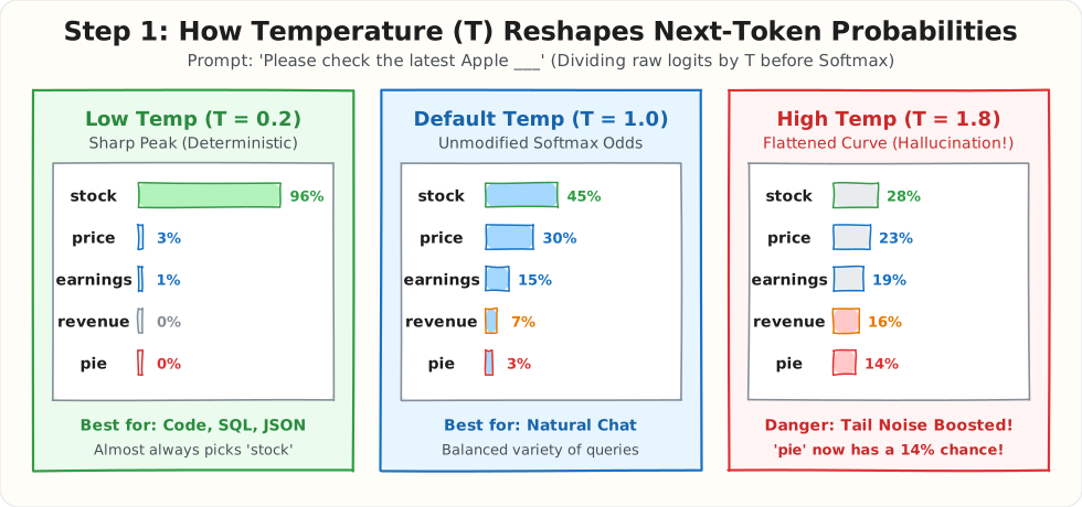
Look at the three panels in the diagram:
- When \(T = 1.0\) (Default): Dividing by 1.0 changes nothing. "stock" gets 45%, "price" gets 30%, "earnings" gets 15%, "revenue" gets 7%, and "pie" gets 3%.
- When \(T = 0.2\) (Low Temperature): Dividing by 0.2 is the same as multiplying every logit by 5 (stock jumps from 3.2 to 16.0, while price becomes 14.0). Because \(e^{16}\) is vastly larger than \(e^{14}\), "stock" captures 96% of the probability mass, and "pie" drops to 0.00001%. As \(T \to 0\), the model becomes Greedy and picks the #1 token every time.
- When \(T = 1.8\) (High Temperature): Dividing by 1.8 squashes the logits closer together (stock becomes 1.77, pie becomes 0.27). Now the bars flatten out: "stock" drops to 28%, and "pie" jumps to a dangerous 14% chance!
That reveals the fundamental flaw of using high Temperature alone: making the model "more creative" by raising Temperature also boosts the long tail of 199,990 completely wrong words.
What Happens to Zero (\(0.0\)) and Negative Logits Under Temperature?
A common question is: What happens when you divide a 0.0 or negative logit by Temperature?
Recall that every logit is divided by \(T\) before exponentiating: \(e^{z_i / T}\).
| Token | Raw Logit (\(z\)) | Default: \(T = 1.0\) | Low Temp: \(T = 0.2\) (Code/Facts) | High Temp: \(T = 1.8\) (Chaos/Hallucination) |
|---|---|---|---|---|
"stock" |
+3.2 |
52.7% | 88.1% (soars) | 41.7% (drops) |
"price" |
+2.8 |
35.3% | 11.9% | 33.4% |
"earnings" |
+1.5 |
9.6% | 0.02% | 16.2% |
"pie" (Zero Logit) |
0.0 |
2.1% | 0.000% (crushed) | 7.0% (inflates 3x!) |
"banana" (Negative Logit) |
-2.5 |
0.18% | 0.000% (erased to zero) | 1.8% (inflates 10x!) |
Two critical engineering insights emerge:
1. Why zero logits get crushed at low \(T\): At \(T = 0.2\), the top word (stock, \(3.2\)) becomes \(3.2 / 0.2 = +16.0\) (\(e^{16} \approx 8.8 \text{ million}\)). The zero word (pie, \(0.0\)) remains \(0.0 / 0.2 = 0.0\) (\(e^0 = 1.0\)). Compared to 8.8 million, a score of 1.0 becomes 0.000%. Low temperature lets the top candidate completely swallow neutral words.
2. Why negative logits trigger hallucinations at high \(T\): At \(T = 1.8\), dividing by \(1.8\) pulls all numbers closer to zero. Negative logit banana (\(-2.5\)) becomes \(-2.5 / 1.8 = -1.39\) (\(e^{-1.39} \approx 0.25\)), inflating its probability from \(0.18\%\) to nearly \(2\%\)! In a 100-word response, that means the AI is almost guaranteed to hallucinate an unrelated word.
3. Truncating the Tail: Fixed Top-K vs. Dynamic Top-P (Nucleus Sampling)
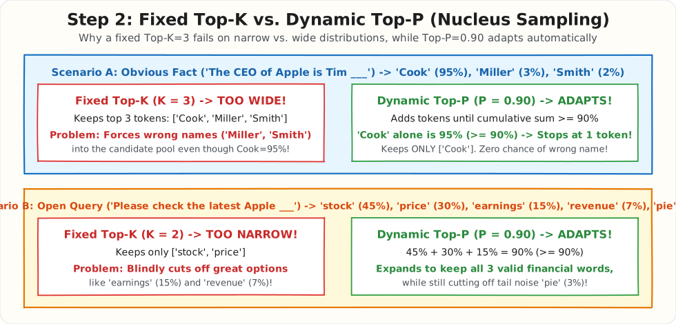
To let the AI use creative variety without ever picking wild words like "pie", we need to chop off the tail of low-probability words before rolling the dice.
Engineers use two different filters for this: Top-K and Top-P.
The Everyday Analogy: The Nightclub Bouncer
Imagine the candidate words are people waiting in line outside a club:
- Top-K is a bouncer with a strict headcount rule:
"Only the first 3 people in line get in. Exactly 3, no matter who they are."
-
The Problem: If person #1 is the only valid VIP ("Cook" at 95%), the bouncer still lets the next 2 strangers in anyway. But if 5 great guests show up, the bouncer cruelly locks 2 of them out.
-
Top-P is a bouncer with a quality threshold:
"Let people in until they make up 90% of the VIP table. If 1 person fills 90%, only 1 gets in. If 3 people are needed to reach 90%, all 3 get in. But never let in the bottom 10% troublemakers."
Side-by-Side: What is the Difference Between Top-K and Top-P?
| Feature | Top-K (Fixed Headcount) | Top-P (Dynamic Quality Bar) |
|---|---|---|
| How it filters | Counts a fixed number of tokens (\(K\)) | Sums up probabilities until they hit threshold \(P\) |
| Candidate pool size | Rigid (always \(K\) words, e.g., exactly 3) | Dynamic (shrinks to 1 word, or expands to 5+ words) |
| When there is only 1 obvious answer (e.g., "The CEO of Apple is Tim ___") |
❌ Too Loose: If \(K=3\), it keeps "Cook" (95%), but is forced to also keep "Miller" (3%) and "Smith" (2%), giving the AI a 5% chance of hallucinating. |
✅ Adapts: "Cook" alone is 95% (\(\ge 90\%\)), so it stops immediately at 1 word. Zero chance of picking "Miller". |
| When multiple answers are valid (e.g., "Please check the latest Apple ___") |
❌ Too Rigid: If \(K=2\), it only keeps "stock" and "price", blindly chopping off "earnings" (15%) even though it is completely valid! |
✅ Adapts: Adds "stock" (45%) + "price" (30%) + "earnings" (15%) = 90%. It keeps all 3 valid words and cuts off "pie" (3%). |
Step-by-Step Walkthrough with Alex's Prompt
Let's see how both filters handle Alex's prompt:
"Please check the latest Apple ___"
The AI model calculates these 5 probabilities:
* "stock" ➔ 45%
* "price" ➔ 30%
* "earnings" ➔ 15%
* "revenue" ➔ 7%
* "pie" ➔ 3%
How Fixed Top-K (K = 2) Handles It:
Alex sets Top-K = 2. The engine sorts the list and strictly keeps only the top 2 words: ["stock", "price"].
* The Flaw: "earnings" is a perfectly normal 15% financial query, but Top-K = 2 locked it out because of an arbitrary headcount rule.
How Dynamic Top-P (P = 0.90) Handles It:
Alex sets Top-P = 0.90 (also called Nucleus Sampling, introduced by Holtzman et al. in 2019). The engine starts from the highest score and adds words one by one into the "nucleus" bucket until their combined probability reaches or exceeds 90%:
- Check
"stock"(45%): Running sum =45%(Under 90% ➔ keep going) - Add
"price"(30%): Running sum = \(45\% + 30\% =\)75%(Under 90% ➔ keep going) - Add
"earnings"(15%): Running sum = \(75\% + 15\% =\)90%➔ Target reached! Cut off immediately. - Discard remaining tail:
"revenue"(7%) and"pie"(3%) are dropped to0%.
Top-P dynamically selected exactly 3 words ("stock", "price", "earnings"), perfectly protecting Alex's financial bot from blurting out "Apple pie".
4. The Exact Internal Execution Order
A common question in interviews and debugging sessions is: "If Temperature, Top-K, Top-P, and Penalties are all enabled, which one runs first?"
Inside production inference engines (vLLM, llama.cpp, TensorRT-LLM, and frontier APIs), every token step executes in this exact 6-stage pipeline:
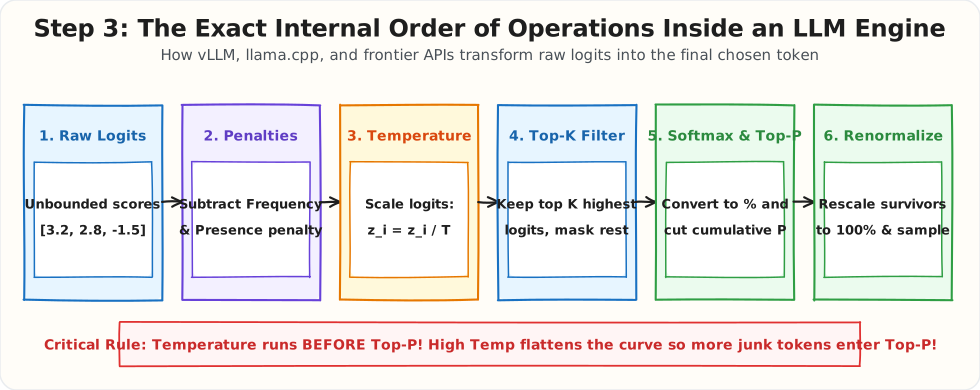
- Raw Logits (\(z\)): Model outputs 200,000 raw scores.
- Repetition / Frequency / Presence Penalties: Engine reduces the logits of tokens that have already appeared in the text.
- Temperature Scaling (\(z_i / T\)): Logits are divided by \(T\). (If \(T = 0\), the engine short-circuits right here and picks \(\arg\max(z)\)).
- Top-K Filter: Only the top \(K\) highest logits are kept; all others are set to \(-\infty\).
- Softmax + Top-P (Nucleus) Filter: Surviving logits are converted to probabilities via Softmax, sorted descending, and cut off once cumulative sum \(\ge P\).
- Renormalization & Weighted Roll: Surviving probabilities are divided by their new sum so they total
100%, and a random number \(r \in [0, 1)\) picks the winning token.
Running the Experiment: Tracing the Sampling Pipeline in Python
Let's run Alex's standalone Python script using numpy to trace how the exact same 5 raw logits ([3.2, 2.8, 2.1, 1.3, 0.5]) behave under different Temperature, Top-K, and Top-P settings.
Click to expand the runnable Python simulation and terminal output
import numpy as np

vocab = ["stock", "price", "earnings", "revenue", "pie"]
raw_logits = np.array([3.2, 2.8, 2.1, 1.3, 0.5])

def sample_pipeline(
    logits: np.ndarray,
    temperature: float = 1.0,
    top_k: int | None = None,
    top_p: float = 1.0,
) -> dict[str, float]:
    # Greedy shortcut for Temperature = 0
    if temperature == 0.0:
        winner = int(np.argmax(logits))
        return {vocab[i]: (1.0 if i == winner else 0.0) for i in range(len(vocab))}

    # Step 1: Temperature scaling
    scaled = logits / temperature

    # Step 2: Top-K filter
    if top_k is not None and top_k < len(scaled):
        cutoff_index = np.argsort(scaled)[-top_k]
        scaled = np.where(scaled >= scaled[cutoff_index], scaled, -np.inf)

    # Step 3: Softmax (subtract max for numerical stability)
    exp_scores = np.exp(scaled - np.max(scaled))
    probs = exp_scores / np.sum(exp_scores)

    # Step 4: Top-P (Nucleus) filter
    if top_p < 1.0:
        sorted_indices = np.argsort(probs)[::-1]
        sorted_probs = probs[sorted_indices]
        cumulative_probs = np.cumsum(sorted_probs)

        # Mask tokens after cumulative sum crosses top_p
        # Shift right by 1 so the token that crosses the threshold is INCLUDED
        cutoff_mask = (cumulative_probs - sorted_probs) >= top_p
        probs[sorted_indices[cutoff_mask]] = 0.0

    # Step 5: Renormalize surviving tokens to sum to 100%
    probs = probs / np.sum(probs)
    return {vocab[i]: round(float(probs[i]), 4) for i in range(len(vocab))}

print("1. Default (T=1.0, P=1.0) :", sample_pipeline(raw_logits, temperature=1.0, top_p=1.0))
print("2. Low Temp (T=0.2, P=1.0):", sample_pipeline(raw_logits, temperature=0.2, top_p=1.0))
print("3. High Temp (T=1.8, P=1.0):", sample_pipeline(raw_logits, temperature=1.8, top_p=1.0))
print("4. Nucleus  (T=1.0, P=0.85):", sample_pipeline(raw_logits, temperature=1.0, top_p=0.85))
Terminal Output:
1. Default (T=1.0, P=1.0) : {'stock': 0.4465, 'price': 0.2993, 'earnings': 0.1486, 'revenue': 0.0668, 'pie': 0.0300}
2. Low Temp (T=0.2, P=1.0): {'stock': 0.8756, 'price': 0.1186, 'earnings': 0.0056, 'revenue': 0.0001, 'pie': 0.0}
3. High Temp (T=1.8, P=1.0): {'stock': 0.3405, 'price': 0.2727, 'earnings': 0.1849, 'revenue': 0.1184, 'pie': 0.0759}
4. Nucleus  (T=1.0, P=0.85): {'stock': 0.4992, 'price': 0.3347, 'earnings': 0.1661, 'revenue': 0.0,    'pie': 0.0}
Look at row 4 (Nucleus T=1.0, P=0.85):
* Before Top-P, "stock" (44.65%) + "price" (29.93%) + "earnings" (14.86%) = 89.44%, which crosses the 85% (0.85) threshold.
* Top-P deletes "revenue" (0.0) and "pie" (0.0), and renormalizes the 3 valid words to 49.92%, 33.47%, and 16.61%.
Where It Fails in Production (Three Classic Sampling Traps)
Click to expand: Three Classic Sampling Traps and Common Developer Mistakes
When moving from a local script to a live backend service, engineers frequently run into three classic sampling traps that degrade output quality or crash parsers:
Failure 1: Tuning Both Temperature and Top-P Together
Developers often set temperature = 1.4 (wanting high creativity) and top_p = 0.5 (wanting high safety) in the same API call.
Look back at our 6-stage pipeline in Step 3: Temperature runs BEFORE Top-P.
1. Setting temperature = 1.4 flattens the probability distribution, stealing probability mass from the best words ("stock", "price") and spreading it into the long tail.
2. Immediately afterward, top_p = 0.5 chops off half the flattened distribution, leaving you with a weird, muddy middle ground where the model has high randomness among mediocre tokens.
That is why OpenAI, Anthropic, and Google explicitly state in their API docs: Alter either temperature OR top_p, never both.
Failure 2: How frequency_penalty Silently Destroys JSON and Code
In conversational text, models sometimes get stuck in repetitive loops:
"Apple stock price is rising because Apple stock price is rising because..."
To stop this repetition, LLM APIs provide a dial called frequency_penalty. The idea sounds simple: every time the model repeats a word, the engine penalizes that token so the model is forced to choose fresh vocabulary.
Alex turns on frequency_penalty = 1.5 to keep answers punchy and non-repetitive, and asks the model to extract Apple's quarterly earnings into a structured JSON array.
Within minutes, Alex's production backend crashes with JSONDecodeError on every incoming request. Why?
How frequency_penalty Calculates Its Punishment
During text generation, the inference engine maintains a running counter for every token generated so far. Before calculating Softmax probabilities, it subtracts a penalty directly from the token's raw score (logit):
If frequency_penalty = 1.5, look at how rapidly the penalty escalates each time a token appears:
| Token Usage Count | Penalty Calculation | Total Subtracted from Raw Logit | Effect on Token's Probability |
|---|---|---|---|
| 1st time (brand new token) | \(1.5 \times 0\) | 0.0 |
Normal probability |
| 3rd time | \(1.5 \times 2\) | -3.0 |
Probability cut by ~95% |
| 6th time | \(1.5 \times 5\) | -7.5 |
Probability crushed to < 0.1% |
| 10th time | \(1.5 \times 9\) | -13.5 |
Practically zero (\(e^{-13.5} \approx 0.000001\)) |
Why Valid JSON Is Impossible Under a Frequency Penalty
Now look at what valid JSON actually requires:
[
  {"metric": "revenue", "value": "$94.9B"},
  {"metric": "net_profit", "value": "$14.7B"},
  {"metric": "gross_margin", "value": "46.2%"}
]
To produce valid syntax, the LLM cannot avoid repeating the exact same structural characters dozens of times:
- The double quote (") appears 18 times in just three metrics.
- The curly braces ({ and }) appear 6 times.
- The colon (:) and comma (,) appear 9 times.
- Schema keys like "metric" and "value" repeat on every single line.
The Exact Moment Generation Breaks
By the time the model finishes generating the second entry (net_profit), it has already used the double quote token (") 12 times.
The model now arrives at the end of the third entry: {"metric": "gross_margin", "value": "46.2%
At this exact step, the model must output a double quote (") to close the value string "46.2%".
- The Model's Raw Logit: The attention layers know that closing a string requires a quote. It assigns the raw logit for
"a strong score of+6.0. - The Penalty Hits: The engine checks its counter: “You have already used
"12 times. Subtracting \(1.5 \times 12 = 18.0\).” - The Adjusted Logit: $\(\text{New Logit} = 6.0 - 18.0 = -12.0\)$
- The Syntax Crash: A logit of
-12.0has a probability of less than \(0.00001\%\). The double quote is mathematically forbidden from winning!
Unable to pick ", the model picks whatever unpenalized token is left—such as a single quote ('), an exclamation mark (!), or a random letter:
[
  {"metric": "revenue", "value": "$94.9B"},
  {"metric": "net_profit", "value": "$14.7B"},
  {"metric": "gross_margin", "value": "46.2%'   <-- Syntax error: single quote used instead!
Worse, when the model attempts to close the object with }, that brace has also been used multiple times and is heavily penalized. The model cannot close the JSON object, causing it to emit unclosed brackets or truncate mid-sentence:
Frequency Penalty vs. Presence Penalty (The Difference)
LLM APIs provide two repetition controls. Here is how they differ:
- Frequency Penalty: Scales with every repetition (\(1.5 \times \text{count}\)). The more you use a token, the harsher the punishment. This is great for creative writing where you want to stop the model from repeating words like "amazing" 10 times, but fatal for JSON, SQL, and code.
- Presence Penalty: A flat, one-time penalty applied once a token appears at least once (\(1.5 \times 1\)), regardless of whether it appeared 1 time or 100 times. It encourages the model to introduce new topics rather than penalizing syntax structure.
Production Rule: Never set
frequency_penalty > 0orpresence_penalty > 0on tasks generating JSON, YAML, SQL, or code. Always leave both at0.0.
Failure 3: Why Temperature = 0.0 Still Produces Different Outputs on Cloud GPUs
Alex set temperature = 0.0 (and even passed a seed = 42 parameter), expecting 100% identical outputs on every single test run. Yet 1 out of 20 runs still differed slightly!
Why isn't Temperature = 0 strictly deterministic on cloud APIs?
1. Floating-Point Non-Associativity on GPUs: In IEEE 754 floating-point math, \((a + b) + c \neq a + (b + c)\) due to tiny rounding differences in parallel GPU thread reductions.
2. Continuous Dynamic Batching: Production LLM servers batch Alex's request together with other users' requests dynamically. If call #1 runs in a batch of size 4 and call #2 runs in a batch of size 19, the GPU kernel chooses a different matrix-multiplication tile size, shifting two tied logits from 3.100001 vs. 3.100002 and flipping the winning token.
3. Mixture-of-Experts (MoE) Routing Ties: In MoE frontier models, tiny floating-point shifts can route a token to a different expert when capacity buffers are full.
[!WARNING] Common Developer Mistakes to Avoid - Using
frequency_penalty > 0on structured outputs (JSON, SQL, Python code): Code and JSON require repeating brackets, quotes, and schema keys. Always keepfrequency_penalty = 0.0andpresence_penalty = 0.0for structured tasks. - Passingtemperatureto Reasoning / Thinking Models: Modern reasoning models (like OpenAI's o-series / reasoning mode or Claude Extended Thinking) manage their own search diversity internally and will either ignoretemperatureor throw a400 Bad Requesterror if you settemperature != 1.0. - Relying ontemperature = 0for security or schema validation: Even attemperature = 0, an LLM can output invalid JSON on weird inputs. Use Structured Outputs (Constrained Decoding) for schema guarantees, not just low temperature.
How to Prevent Sampling Failures in Production
Click to expand: Task-Bound Sampling Profiles in Code
To prevent these failures, production systems should never use one global set of sampling parameters across all features. Instead, Alex defines Task-Bound Sampling Profiles in code, tailored to each endpoint:
from dataclasses import dataclass

@dataclass(frozen=True)
class SamplingConfig:
    temperature: float
    top_p: float
    frequency_penalty: float = 0.0
    presence_penalty: float = 0.0

# 1. Strict deterministic profile for JSON, SQL, and Tool Calling
STRICT_DATA_PROFILE = SamplingConfig(
    temperature=0.0,
    top_p=1.0,
    frequency_penalty=0.0,  # Never penalize repeated JSON keys or brackets!
    presence_penalty=0.0,
)

# 2. Grounded profile for Customer Support RAG Q&A
GROUNDED_QA_PROFILE = SamplingConfig(
    temperature=0.2,        # Slight warmth for natural phrasing, near-zero tail risk
    top_p=1.0,              # Leave top_p at 1.0 since temperature is tuned
)

# 3. Creative profile for Marketing & Brainstorming
CREATIVE_COPY_PROFILE = SamplingConfig(
    temperature=1.0,        # Keep temperature neutral
    top_p=0.90,             # Use Nucleus Sampling to allow diverse words safely
    presence_penalty=0.3,   # Gentle nudge toward fresh vocabulary
)
What Does It Cost? (Engineering Trade-Offs)
Unlike context window length, changing Temperature or Top-P costs zero extra dollars per token, but it dramatically changes error rates, retry costs, and caching efficiency:
| Sampling Strategy | Compute Overhead per Token | Output Cacheability | Schema / Fact Reliability | Diversity & Creativity | Hidden Production Cost |
|---|---|---|---|---|---|
Greedy (Temp = 0.0, Top-P = 1.0) |
~0.01 ms (Fastest: argmax only, skips Softmax) |
High (Same input hits response cache) | 99.2% (Lowest hallucination rate) | Lowest (Can loop on long essays) | Near zero retry cost |
Low Temp (Temp = 0.2, Top-P = 1.0) |
~0.05 ms |
Medium | 98.5% | Balanced natural phrasing | Standard for RAG chat |
Nucleus (Temp = 1.0, Top-P = 0.90) |
~0.12 ms (Requires full sort of 200K vocab) |
Low (Every run is unique) | 91.0% | High (Rich vocabulary without tail garbage) | Higher validation retries if used on data tasks |
High Temp (Temp = 1.5, Top-P = 1.0) |
~0.05 ms |
Zero | < 65% (Frequent hallucinations) | Chaotic | High retry bill from failed JSON/hallucinations |
Production Design: Task-Specific Sampling Router
In production AI systems, sampling parameters are never hardcoded globally in an environment variable (LLM_TEMP=0.7). Instead, the AI Gateway routes each request to a specific sampling profile based on the endpoint's job:
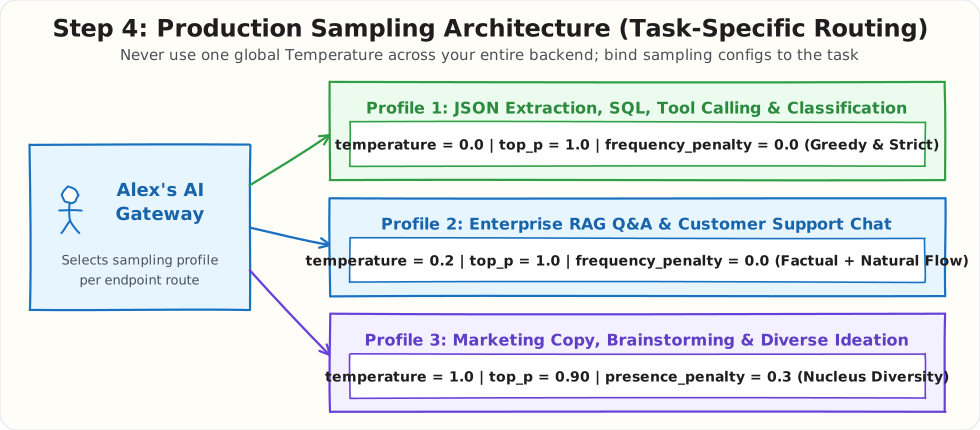
- Data & Tool Endpoints (
/extract-order,/generate-sql): Locked totemperature = 0.0, top_p = 1.0, frequency_penalty = 0.0paired with a JSON Schema constraint. - RAG & Support Endpoints (
/chat-support): Usestemperature = 0.2, top_p = 1.0so the bot stays faithful to retrieved documents without sounding robotic. - Ideation & Copywriting Endpoints (
/draft-campaign): Usestemperature = 1.0, top_p = 0.90, presence_penalty = 0.3to explore diverse phrasing while cutting off the bottom 10% tail.
When to Use vs. When NOT to Use
| Parameter / Setting | When to Use in Production | When NOT to Use (And What to Do Instead) |
|---|---|---|
temperature = 0.0 |
✅ Code generation, SQL queries, JSON extraction, classification, math, and unit-testable pipelines. | ❌ Creative writing, brainstorming, or generating 5 diverse variations of a headline (all 5 will be identical!). |
top_p = 0.90 (with temp = 1.0) |
✅ Open-ended chat, marketing copy, storytelling, and dialogue where natural variety matters. | ❌ When you are already tuning temperature = 0.2. Tune one or the other, not both. |
top_k (e.g., K = 40) |
✅ Local open-weight models (llama.cpp / vLLM) as a fast pre-filter before top_p so the CPU/GPU only sorts 40 items instead of 200,000. |
❌ As your only filter on factual Q&A (fixed K=40 lets 39 wrong answers into the pool when only 1 answer is right). |
presence_penalty (0.1 – 0.5) |
✅ Long creative articles or multi-turn roleplay where the model keeps repeating the same adjectives. | ❌ Summarizing a technical document (where key domain terms must be repeated accurately) or generating code/JSON. |
Interview Questions & Curveballs
1. "Why is Top-P (Nucleus Sampling) generally preferred over Top-K in modern LLMs?"
- How to answer:
Top-Kuses a fixed bucket size (\(K\)), which fails when the entropy of the next token changes. On a factual token where one word has 95% probability,Top-K = 10forces 9 wrong words into the sample pool. On an open-ended token where 20 adjectives are equally good at 4% each,Top-K = 10arbitrarily cuts off half of the good words.Top-Psets a cumulative probability threshold (such as 90%), shrinking the pool to 1 token on confident facts and expanding it to 20 tokens on creative choices.
2. "In what order are Temperature, Top-K, and Top-P applied to logits, and why does the order matter?"
- How to answer: The order is
Repetition Penalties ➔ Temperature Scaling ➔ Top-K ➔ Softmax ➔ Top-P ➔ Renormalize. Because Temperature runs before Top-P, changing Temperature changes how many tokens survive the Top-P cutoff. Raising Temperature flattens the probability distribution, which forces Top-P to include many more low-quality tail tokens to reach the 90% sum.
3. "If I set Temperature = 0, why does Greedy Decoding not need to compute Softmax at all?"
- How to answer: Softmax (\(e^{z_i} / \sum e^{z_j}\)) is a monotonically increasing function, meaning the token with the highest raw logit \(z_i\) is guaranteed to have the highest Softmax probability. At
Temperature = 0, the engine simply takes \(\arg\max(z)\) directly on the raw logits, skipping the expensive exponential sum across 200,000 tokens.
4. "Why does Temperature = 0 still occasionally return different responses across API calls?"
- How to answer: GPU floating-point addition and matrix multiplication are non-associative. When a cloud inference server uses Continuous Batching, your request is grouped with a varying number of concurrent requests on each run. Different batch sizes trigger different CUDA kernel split-K reductions, causing microscopic \(10^{-7}\) floating-point variations that can flip the winner when two tokens have nearly identical logits.
Summary Cheat Sheet
| Parameter | Formula / Mechanism | Default Value | Lower Value Effect | Higher Value Effect | Production Rule of Thumb |
|---|---|---|---|---|---|
| Temperature (\(T\)) | Divides raw logits: \(z_i / T\) | 1.0 |
Sharpens peak; 0.0 = Greedy (\(\arg\max\)) |
Flattens curve; boosts rare tail tokens | Use 0.0 for code/JSON, 0.2 for RAG, 0.8–1.0 for creative tasks |
| Top-P (Nucleus) | Keeps smallest set of top tokens where \(\sum P \ge p\) | 1.0 |
Restricts pool to only the highest-confidence core | Includes more of the long tail (1.0 = all tokens) |
Use 0.90–0.95 when Temp = 1.0; leave at 1.0 if tuning Temp |
| Top-K | Keeps only the top \(K\) highest-ranked tokens | Disabled / None |
Strictly limits candidate count to \(K\) | Allows more candidates into Softmax | Useful as a fast pre-filter (K = 50) in local engines (vLLM) |
| Frequency Penalty | Subtracts \(\alpha \times \text{count}_i\) from logit | 0.0 |
Allows natural repetition | Strongly punishes words proportional to usage count | Keep at 0.0 for JSON/code so brackets & keys aren't blocked |
| Presence Penalty | Subtracts flat \(\alpha\) if \(\text{count}_i > 0\) | 0.0 |
Stays focused on current topic | Nudges model to introduce new topics/words | Use 0.1–0.3 for brainstorming; 0.0 for factual RAG |
What's Next?
Setting temperature = 0.0 makes the model pick the highest-probability token at each step, but it still does not guarantee that the model will follow instructions or return 100% valid JSON when a customer types a weird or adversarial message!
In our next guide (Topic #4: From Prompt Engineering to Context Engineering & Structured Outputs), we will see how modern Context Engineering structures system instructions and how Constrained Decoding masks invalid tokens right inside the sampling pipeline so your JSON schemas never break in production.